scikit-learnによる機械学習プログラミング入門

前処理：データの準備

scikit-learnに同梱されているirisデータセットを使う。

from sklearn import datasets
import numpy as np

iris = datasets.load_iris()
print(iris.DESCR)

.. _iris_dataset:

Iris plants dataset
--------------------

**Data Set Characteristics:**
...

irisデータセットの中身を見る。

import pandas as pd
iris_df = pd.DataFrame(iris.data, columns=iris.feature_names)
iris_df['species'] = [iris.target_names[i] for i in iris.target]

iris_df.sample(10)

	sepal length (cm)	sepal width (cm)	petal length (cm)	petal width (cm)	species
1	4.9	3.0	1.4	0.2	setosa
124	6.7	3.3	5.7	2.1	virginica
147	6.5	3.0	5.2	2.0	virginica
95	5.7	3.0	4.2	1.2	versicolor
39	5.1	3.4	1.5	0.2	setosa
19	5.1	3.8	1.5	0.3	setosa
42	4.4	3.2	1.3	0.2	setosa
27	5.2	3.5	1.5	0.2	setosa
18	5.7	3.8	1.7	0.3	setosa
93	5.0	2.3	3.3	1.0	versicolor

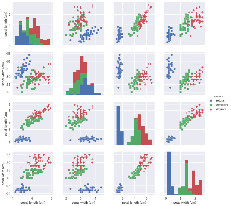
irisデータセットの分布を眺める。

import seaborn as sns
sns.pairplot(iris_df, hue='species', markers=["o", "s", "D"])

png

特徴選択：petal lengthとpetal width ([2, 3]) を特徴量として使うことにする。

X = iris.data[:, [2, 3]]
y = iris.target

print('Class labels:', np.unique(y))

Class labels: [0 1 2]

前処理：データの分割

トレーニングデータとテストデータに分割する。

from sklearn.model_selection import train_test_split

X_train, X_test, y_train, y_test = train_test_split(
    X, y, test_size=0.3, random_state=1, stratify=y)
print('Labels counts in y:', np.bincount(y))
print('Labels counts in y_train:', np.bincount(y_train))
print('Labels counts in y_test:', np.bincount(y_test))

Labels counts in y: [50 50 50]
Labels counts in y_train: [35 35 35]
Labels counts in y_test: [15 15 15]

前処理：スケーリング

StandardScalerを使って、平均0 分散1となるようにデータをスケーリングする。

from sklearn.preprocessing import StandardScaler

sc = StandardScaler()
sc.fit(X_train)
X_train_std = sc.transform(X_train)
X_test_std = sc.transform(X_test)

学習：トレーニングデータによる予測モデル学習

パーセプトロンと呼ばれるある学習アルゴリズムにより学習

from sklearn.linear_model import Perceptron

ppn = Perceptron(max_iter=40, tol=1e-3, eta0=0.1, random_state=1234)
ppn.fit(X_train_std, y_train)

Perceptron(alpha=0.0001, class_weight=None, early_stopping=False, eta0=0.1,
      fit_intercept=True, max_iter=40, n_iter=None, n_iter_no_change=5,
      n_jobs=None, penalty=None, random_state=1234, shuffle=True,
      tol=0.001, validation_fraction=0.1, verbose=0, warm_start=False)

他に使用可能なアルゴリズム（一部）

k最近傍法 (sklearn.neighbors.KNeighborsClassifier)
ロジスティック回帰 (sklearn.linear_model.LogisticRegression)
サポートベクタマシン (sklearn.svm.SVC)
ランダムフォレスト (sklearn.ensemble.RandomForestClassifier)

評価：テストデータによる精度評価

テストデータにおける精度（的中率）を計算する。

y_pred = ppn.predict(X_test_std)
print('Misclassified samples: %d' % (y_test != y_pred).sum())

Misclassified samples: 1

from sklearn.metrics import accuracy_score
print('Accuracy: %.2f' % accuracy_score(y_test, y_pred))

Accuracy: 0.98

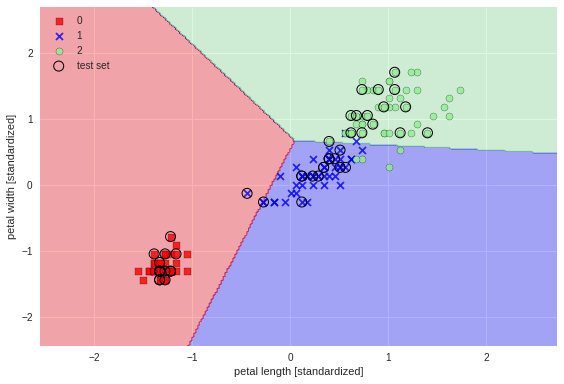
評価：予測モデルの可視化

予測モデルの線形関数を散布図にプロットする。

from matplotlib.colors import ListedColormap
import matplotlib.pyplot as plt


def plot_decision_regions(X, y, classifier, test_idx=None, resolution=0.02):

    # setup marker generator and color map
    markers = ('s', 'x', 'o', '^', 'v')
    colors = ('red', 'blue', 'lightgreen', 'gray', 'cyan')
    cmap = ListedColormap(colors[:len(np.unique(y))])

    # plot the decision surface
    x1_min, x1_max = X[:, 0].min() - 1, X[:, 0].max() + 1
    x2_min, x2_max = X[:, 1].min() - 1, X[:, 1].max() + 1
    xx1, xx2 = np.meshgrid(np.arange(x1_min, x1_max, resolution),
                           np.arange(x2_min, x2_max, resolution))
    Z = classifier.predict(np.array([xx1.ravel(), xx2.ravel()]).T)
    Z = Z.reshape(xx1.shape)
    plt.contourf(xx1, xx2, Z, alpha=0.3, cmap=cmap)
    plt.xlim(xx1.min(), xx1.max())
    plt.ylim(xx2.min(), xx2.max())

    for idx, cl in enumerate(np.unique(y)):
        plt.scatter(x=X[y == cl, 0], 
                    y=X[y == cl, 1],
                    alpha=0.8, 
                    c=colors[idx],
                    marker=markers[idx], 
                    label=cl, 
                    edgecolor='black')

    # highlight test samples
    if test_idx:
        # plot all samples
        X_test, y_test = X[test_idx, :], y[test_idx]

        plt.scatter(X_test[:, 0],
            X_test[:, 1],
            facecolor='none',
            edgecolor='black',
            alpha=1.0,
            linewidth=1,
            marker='o',
            s=100, 
            label='test set')

X_combined_std = np.vstack((X_train_std, X_test_std))
y_combined = np.hstack((y_train, y_test))

plot_decision_regions(X=X_combined_std, y=y_combined,
                      classifier=ppn, test_idx=range(105, 150))
plt.xlabel('petal length [standardized]')
plt.ylabel('petal width [standardized]')
plt.legend(loc='upper left')

plt.tight_layout()

png